Compute the theoretical BER for AWGN channel and various constellation size

Based on the previous skeleton, we can now compute an iterative testbench to compute the Bit Error Rate for various constellation size, and compare the simulation with the theory. As a gentle reminder, the theoretical bit error rate can be approximated as

$\mathrm{BER} = \frac{ 4 \left( 1 - \frac{1}{\sqrt{M}} \right) }{ \log_2(M)} \times Q( \sqrt{ \frac{6 \log_2(M)}{2(M-1)} \frac{Eb}{N_0}}$

First of all let's call the modules

using DigitalComm 
using PGFPlotsX

We define first the main monte-carlo function that compute an elementary Tx-Rx link, and returns the number of error and number of bit computed (to be accumulated)

function monteCarlo(snr,mcs,nbSymb) 
    # Number of bits  
    nbBits    = nbSymb * Int(log2(mcs));
    # --- Binary sequence generation 
    bitSeq    = genBitSequence(nbBits);
    # --- QPSK mapping
    qamSeq    = bitMappingQAM(mcs,bitSeq);
    # ---------------------------------------------------- 
    # --- Channel  
    # ---------------------------------------------------- 
    #  --- AWGN
    # Theoretical power is 1 (normalized constellation)
    qamNoise,  = addNoise(qamSeq,snr,1);
    # ----------------------------------------------------
    # --- Rx Stage: SRRC
    # ----------------------------------------------------
    # --- Binary demapper
    bitDec  = bitDemappingQAM(mcs,qamNoise);
    # --- Error counter 
    nbE     = sum(xor.(bitDec,bitSeq));
    # --- Return Error and bits 
    return (nbE,nbBits);
end

A function to plot the BER versus the SNR, for different mcs and compare to theory

function doPlot(snrVect,ber,qamVect)
    a = 0;
    @pgf a = Axis({
        ymode     = "log",
        height      ="3in",
        width       ="4in",
        grid,
        xlabel      = "SNR [dB]",
        ylabel      = "Bit Error Rate ",
        ymax       = 1,
        ymin       = 10.0^(-5),
        title       = "AWGN BER for QAM",
        legend_style="{at={(0,0)},anchor=south west,legend cell align=left,align=left,draw=white!15!black}"
        },
        Plot({color="red",mark="square*"},Table([snrVect,ber[1,:]])),
        LegendEntry("QPSK"),
        Plot({color="green",mark="*"},Table([snrVect,ber[2,:]])),
        LegendEntry("16-QAM"),

        Plot({color="purple",mark="triangle*"},Table([snrVect,ber[3,:]])),
        LegendEntry("64-QAM"),
        Plot({color="blue",mark="diamond*"},Table([snrVect,ber[4,:]])),
        LegendEntry("256-QAM"),
    );
    # ---  Adding theoretical curve
    snrLin  = (10.0).^(snrVect/10)
    for qamScheme = qamVect
        ebNo    = snrLin / log2(qamScheme);
        # This approximation is only valid for high SNR (one symbol error is converted to one bit error with Gray coding).
        berTheo   = 4 * ( 1 - 1 / sqrt(qamScheme)) / log2(qamScheme) * qFunc.(sqrt.( 2*ebNo * 3 * log2(qamScheme) / (2*(qamScheme-1)  )));
        @pgf push!(a,Plot({color="black"},Table([snrVect,berTheo])));
    end
    display(a);
end

Then, the main routine to compute the BER for a given number of iterations and a range of SNR

function main() 
# --- Parameters 
nbIt            = 10000;          # Number of iterations  
nbSymb          = 1024;           # Number of symbols per iterations 
mcs             = [4,16,64,256];  # Constellation size 
snrRange        = (-1:26);        # SNR, expressed in dB 
# --- Init performance metrics
nbSNR           = length(snrRange);
ber             = zeros(Float64,length(mcs),nbSNR);
for iMcs = 1 : 1  : length(mcs)
    for iSNR = 1 : 1 : nbSNR
        # --- Create BER counters 
        nbE   = 0;
        nbB   = 0;
        for iN = 1 : 1 : nbIt
            # --- Elementary MC call 
            # Corresponds to a given SNR and a given iteration 
            # As we are ergodic in AWGN, it is only nbSymb*nbIt that matters for BER computation
            (a,b) = monteCarlo(snrRange[iSNR],mcs[iMcs],nbSymb); 
            # --- Update counters 
            nbE += a;     # Increment errors 
            nbB += b;     # Increment bit counters 
        end 
        ber[iMcs,iSNR] = nbE / nbB; 
    end
end 
# --- Plotting routine
doPlot(snrRange,ber,mcs);
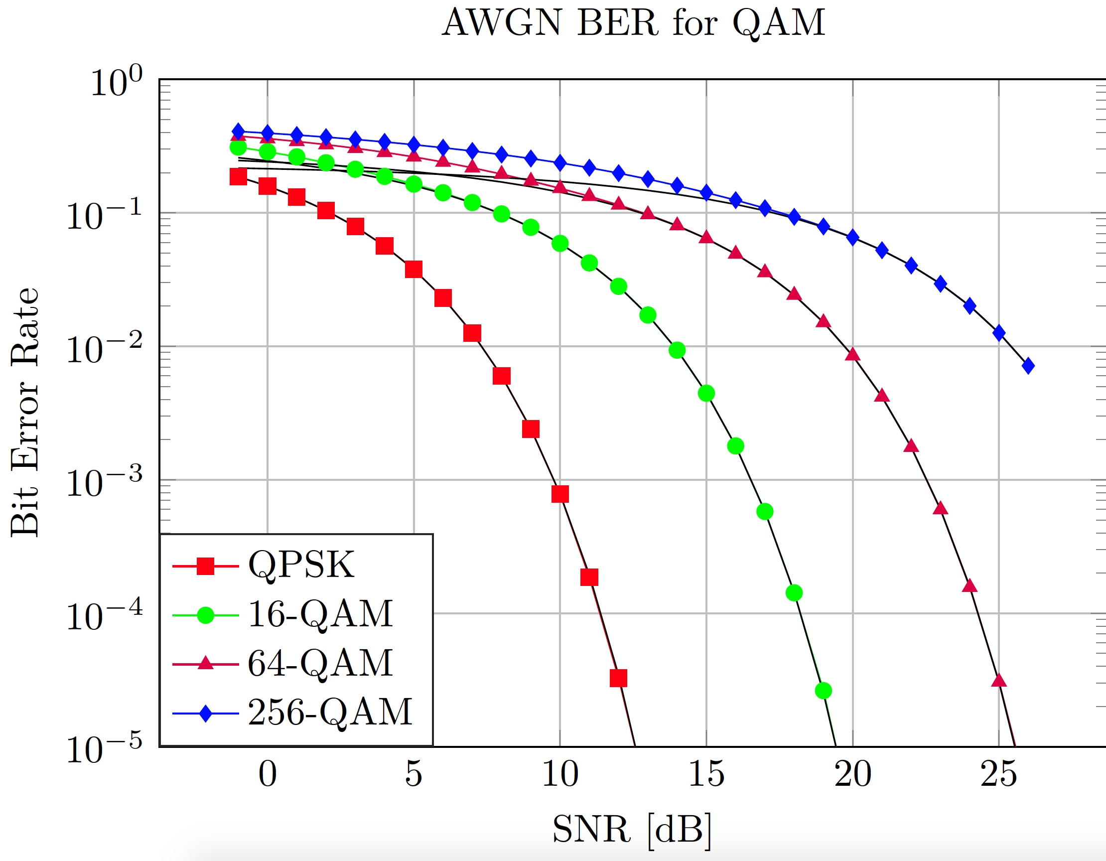
end

The output plot is the following, showing adequacy between theory and practise for high SNR (the theoretical curve is under the assumption that one symbol error leads to one erroneous bit (gray coding) which is true only with intermediate noise levels).